Image Source: DeepLizard Youtube video
📝 Q1: 1) What are the parameters of batchnorm? What information do you need to train the parameters?
2) Why do we use ‘exponentially weighted moving average’ (chain of linear interpolation) of training data optimizing two parameters? In other words, why can’t we use one batch of training set’s mean and variance in inference time?
📝 Q2: Briefly explain advantage and disadvantage of batch normalization.
🎮 Q3: Implement customized batch norm, and plot activations’ mean and std.
🎮 Q4: Use built-in batchnorm of pytorch
🎮 Q5: Add scheduler and train
📝 🎮 Q6: Explain difference between batchnorm and layernorm. Implement Layernorm class.
📝 🎮 Q7: Implement InstanceNorm class. Why do you think the model trained on instance norm can not be a classification model? 1
🎮 Q8: GroupNorm: initialize activation with N=20, channel = 6, height, width = 10 and 1) separate 6 channels into 3 groups 2) separate 6 channels into 6 groups (instancenorm) 3) put all 6 channels into as signle group (layernorm)
📝 🎮 Q9: Fastai introduces RunningBatchNorm class to be used in small batch cases. Implement it and write your opinion for what reason RunningBatchNorm uses smoother means and variacne of small batch size.
- hint: torch.numel(), torch.new_tensor()
A1
1) \(\frac{X - \mu}{\sigma} * \gamma + \beta\), in which \(\gamma\) and \(\beta\) are optimized using training data (i.e. parameter) and \(\mu\) and \(\sigma\) attained from data.
2) When we get a totally different type of image at inference time, we can not fairly access/evaluate the parameters since attained mean/variance of training data are irrevant to inference.
A2
- Advantages
- Learn parameter much faster with bigger learning rate: If you normalize activation(i.e. output of each layer) through batch (using mean, std of previous 2 batches), risk of vanishing/exploding gradient is much less likely to happen. So that you get faster result.
- Disdvantages
- In online learning (batchsize=1) you can not use batch normalization.2
- In segmentation task you can not use batch norm.
- You can not use batchnorm in RNN also since the weight matrix will be shared through layers.
A3
class BatchNorm(nn.Module):
def __init__(self, nf, mom=0.1, eps=1e-6):
super().__init__()
self.mom, self.eps = mom, eps
self.mults = nn.Parameter(torch.ones (nf, 1, 1))
self.adds = nn.Parameter(torch.zeros(nf, 1, 1))
self.register_buffer('vars', torch.ones (1, nf, 1, 1))
self.register_buffer('means', torch.zeros(1, nf, 1, 1))
def update_stats(self, x):
'''first get stats of last 2 batches and then save current m, v with lerp'''
m = x.mean((0, 2, 3), keepdim=True)
v = x.var ((0, 2, 3), keepdim=True)
self.means.lerp_(m, self.mom) # linear interpolation
self.vars.lerp_ (v, self.mom)
# if len(self.means[0])==8: print(f"Training time:\nmean: {m}\nvarience: {v}")
return m, v
def forward(self, x):
if self.training:
with torch.no_grad():
m, v = self.update_stats(x)
else:
m, v = self.means, self.vars # Q. does this mean and variance does not change during inference time? => A. Yes
# if len(self.means[0])==8: print(f"Inference time:\nmean: {m}\nvarience: {v}")
# ipdb.set_trace()
x = (x-m) / (v+self.eps).sqrt()
return x*self.mults + self.adds
def conv_layer(ni, nf, ks=3, stride=2, bn=True, **kwargs):
layers = [nn.Conv2d(ni, nf, ks, padding=ks//2, stride=stride, bias=not bn),
GeneralRelu(**kwargs)]
if bn: layers.append(BatchNorm(nf))
return nn.Sequential(*layers)
def init_cnn_(m, f):
if isinstance(m, nn.Conv2d):
f(m.weight, a=0.1)
if getattr(m, 'bias', None) is not None: m.bias.data.zero_()
for l in m.children(): init_cnn_(l, f)
def init_cnn(m, uniform =False):
f = init.kaiming_uniform_ if uniform else init.kaiming_normal_
init_cnn_(m, f)
def get_learn_run(nfs, data, lr, layer, cbs=None, opt_func=None, uniform=False, **kwargs):
model = get_cnn_model(data, nfs, layer, **kwargs)
init_cnn(model, uniform=uniform)
return get_runner(model, data, lr=lr, cbs=cbs, opt_func=opt_func)
learn, run = get_learn_run(nfs, data, 0.9, conv_layer, cbs=cbfs)
with Hooks(learn.model, append_stats) as hooks:
run.fit(1, learn)
fig, (ax0, ax1) = plt.subplots(1, 2, figsize=(10, 4))
for h in hooks[:-1]:
means, stds = h.stats
ax0.plot(means[:20])
ax0.title.set_text('means, batch 20')
ax1.plot(stds[:20])
ax1.title.set_text('stds, batch 20')
h.remove() # [^1]
plt.legend(range(5))
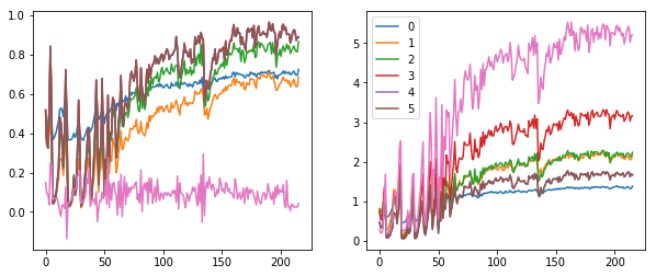
# all batches
fit, (ax0, ax1) = plt.subplots(1, 2, figsize=(10, 4))
ax0.title.set_text('means, all batch')
ax1.title.set_text('stds, all batch')
for h in hooks[:-1]:
means, stds = h.stats
ax0.plot(means)
ax1.plot(stds)
A4
def conv_layer(ni, nf, ks=3, stride=2, bn=True, **kwargs):
    layers = [nn.Conv2d(ni, nf, ks, padding=ks//2, stride=stride, bias = not bn)]
    if bn: layers.append(nn.BatchNorm2d(nf))
    return nn.Sequential(*layers)

learn, run = get_learn_run(nfs, data, 1., conv_layer, cbs=cbfs)
run.fit(3, learn)
A5
sched = combine_scheds([0.3, 0.7], [sched_lin(0.6, 2.), sched_lin(2., 0.1)])
learn, run = get_learn_run(nfs, data, 0.9, conv_layer, cbs=cbfs+[partial(ParamScheduler, 'lr', sched)])
run.fit(1, learn)
run.recorder.plot_lr()
A6
Layernorm does not use moving average, since it’s for online-learning or when batchsize is very small. And layernorm average over hidden dimension, not batch.
class LayerNorm(nn.Module):
    __constants__ = ['eps']
    def __init__(self, eps = 1e-6):
        super().__init__()
        self.eps = eps
        self.mult = nn.Parameter(tensor(1.))
        self.add  = nn.Parameter(tensor(0.))
    def forward(self, x):
        m = x.mean((1, 2, 3), keepdim=True)
        v = x.var ((1, 2, 3), keepdim=True)
        x = (x-m) / (v + self.eps).sqrt()
        return x*self.mult + self.add

def conv_ln(ni, nf, ks=3, stride=2, bn=True, **kwargs):
    layers = [nn.Conv2d(ni, nf, ks, padding=ks//2, stride=stride, bias = True),
              GeneralRelu(**kwargs)]
    if bn: layers.append(LayerNorm())
    return nn.Sequential(*layers)

learn, run = get_learn_run(nfs, data, 1., conv_layer, cbs=cbfs)
run.fit(3, learn)
A7
class InstanceNorm(nn.Module):
    __constants__ = ['eps']
    def __init__(self, nf, eps = 1e-0):
        super().__init__()
        self.eps = eps
        self.mults = nn.Parameter(torch.ones (nf, 1, 1))
        self.adds  = nn.Parameter(torch.zeros(nf, 1, 1))

    def forward(self, x):
        m = x.mean((2, 3), keepdim = True)
        v = x.var((2, 3), keepdim = True)
        res = (x-m) / (v+self.eps).sqrt()
        return res * self.mults + self.adds

def conv_in(ni, nf, ks = 3, stride = 2, bn = True, **kwargs):
    layers = [nn.Conv2d(ni, nf, ks, padding=ks//2, stride=stride, bias = True),
              GeneralRelu(**kwargs)]
    if bn: layers.append(InstanceNorm(nf))
    return nn.Sequential(*layers)
learn, run = get_learn_run(nfs, data, 0.1, conv_in, cbs=cbfs)
run.fit(3, learn)
- Model learns parameter to normalize the contrast within image, which is adequate to, for example, style transferring, since it tunes img color spectrum in one image. Classification is for finding common pattern between images so that model recognizes specific pattern given image.
A8
input = torch.randn(20, 6, 10, 10)
nn.GroupNorm(3, 6) # 1)
nn.GroupNorm(6, 6) # 2)
nn.GroupNorm(1, 6) # 3)
A9
class RunningBatchNorm(nn.Module):
    def __init__(self, nf, mom=0.1, eps=1e-5):
        super().__init__()
        self.mon, self.eps = mom, eps
        self.mults = nn.Parameter(torch.ones (nf,1,1))
        self.adds  = nn.Parameter(torch.zeros(nf,1,1))
        self.register_buffer('sums', torch.zeros(1, nf, 1, 1))
        self.register_buffer('sqrs', torch.zeros(1, nf, 1, 1))
        self.register_buffer('batch', tensor(0.))
        self.register_buffer('count', tensor(0.))
        self.register_buffer('step', tensor(0.))
        self.register_buffer('dbias', tensor(0.))

    def update_stats(self, x):
        bs, nc, *_ = x.shape
        self.sums.detach_()
        self.sqrs.detach_()
        dims = (0, 2, 3)
        s = x.sum(dims, keepdim=True)
        ss = (x*x).sum(dims, keepdim=True)
        c = self.count.new_tensor(x.numel()/nc)
        mom1 = 1 - (1-self.mon)/ math.sqrt(bs-1)
        self.mom1 = self.dbias.new_tensor(mom1)
        self.sums.lerp_(s, self.mom1)
        self.sqrs.lerp_(ss, self.mom1)
        self.count.lerp_(c, self.mom1)
        self.dbias = self.dbias*(1-self.mom1) + self.mom1
        self.batch += bs
        self.step += 1

    def forward(self, x):
        if self.training: self.update_stats(x)
        sums = self.sums
        sqrs = self.sqrs
        c = self.count
        if self.step < 100:
            sums = sums / self.dbias
            sqrs = sqrs / self.dbias
            c  = c / self.dbias
        means = sums/c
        vars = (sqrs/c).sub_(means*means)
        if bool(self.batch < 20): vars.clamp_min_(0.01)
        x = (x-means).div_((vars.add_(self.eps)).sqrt())
        return x.mul_(self.mults).add_(self.adds)

def conv_rbn(ni, nf, ks=3, stride=2, bn =True, **kwargs):
    layers = [nn.Conv2d(ni, nf, ks, padding=ks//2, stride=stride, bias = not bn),
              GeneralRelu(**kwargs)]
    if bn: layers.append(RunningBatchNorm(nf))
    return nn.Sequential(*layers)

learn, run = get_learn_run(nfs, data, 0.4, conv_rbn, cbs = cbfs)
run.fit(1, learn)
- Running batch norm interpolates all elements within arithmetic, for example, if you mean something, RunningBatchNorm interpolates counts, sums not means itself.
 Part2 lesson 10, 06 ConvNet cuda hooks | fastai 2019 course -v3